Ensemble Methods

You have most likely utilized ensemble approaches to avoid overfitting!

Let us discuss what makes ensemble techniques useful and how to prevent frequent mistakes that lead to their abuse in finance.

How can we break down algorithmic errors?

Three errors due to unrealistic assumptions are common in machine learning models. The model fails to detect critical feature-outcome relationships when the bias is significant, resulting in an underfit. Variance error is created by the training set's sensitivity to small movements in the market. When the variance is substantial, the model has overfitted the training set. Therefore even little changes in the training set samples might result in different predictions. When overfitting is present, the noise is calibrated as the signal instead of modeling the patterns in the training data.

Consider a collection of training observations and real-valued outcomes $\left\{(x_i, y_i)\right\}_{i=1}^n$. Assume there is a function $f(x)$ such that:

where $\varepsilon$ is white noise with mean $0$ and standard deviation $\sigma_{\varepsilon}$. We would want to estimate the function $\hat{f}[x]$ that best matches $f(x)$, by minimizing the variance of the estimation error:

This mean-squared error can be broken down as follows:

An ensemble approach is a method that combines a group of weak learners that use the same learning algorithm to build a stronger learner who outperforms all the base learners.

How can model aggregation be used to reduce variance?

Bootstrap aggregation, often known as bagging, is an efficient method for lowering prediction variation. It works like this: To begin, create $N$ training datasets using random sampling with replacement. Second, for each training set, fit $N$ estimators. Because these estimators are trained independently, the models can be fit together. Third, the ensemble prediction is the simple average of the $N$ models' forecasts. For classification problems, the ratio of base estimators that vote for a specific outcome can form a pseudo-probability indicating how likely that label can be assigned to a test set sample. The bagging classifier may calculate the mean of the probabilities when the base estimator provides a probability forecast. For example, assume you have a series of Gaussian Mixture models giving you probabilities that a given sample $x_\text{new}$ can be assigned to any of your $K$ labels. If there is an ensemble of N GMMs, then we can calculate the mean of these probabilities across all the N base estimators.

Let us show mathematically how the bagging method we just discussed reduces variance?

The fundamental advantage of bagging is that it minimizes forecast variance to address overfitting. The variance of the bagged prediction $\left(\varphi_{i}[c]\right)$ varies with the number of base estimators $(N)$, the average variance of a single estimator's prediction $(\bar{\sigma})$, and the average correlation between their predictions $(\bar{\rho})$:

where $\sigma_{i, j}$ is the covariance of predictions by estimators $i, j$, which gives a formula for the average correlation $\bar{\rho}$:

The preceding equation demonstrates that bagging is only helpful to the degree that $\bar{\rho}<$ $1;$ as

One of the benefits of sequential bootstrapping is to generate samples that are as independent as possible, lowering $\bar{\rho}$ and the variance of bagging classifiers.

The standard deviation of the bagged prediction is plotted in this Figure as a function of $N \in[5,30], \bar{\rho} \in[0,1]$ and $\bar{\sigma}=1$.

is Loading ...

How does the bagging classifier's voting mechanism improves accuracy?

Consider a bagging classifier that predicts $k$ classes based on a majority vote among $N$ independent classifiers with a $\{0,1\}$ outcome. A base classifier's accuracy is the probability $p$ of identifying a correct prediction as label 1. We will obtain $N p$ predictions labeled as 1 on average, with a famously known variance of $N p(1-p)$. When a class with the highest votes is observed, majority voting makes an accurate prediction. A sufficient condition is that the total of these labels is greater than $\frac{N}{2}$. A required condition is that $X>\frac{N}{k}$ happens with probability:

The consequence is that given a sufficiently big $N$, say $N>p(p-1 / k)^{-2}$, we have:

and so the bagging classifier's accuracy surpasses the individual classifiers' average accuracy.

This is a compelling case for bagging any classifier in general when computing constraints allow it. Unlike boosting, however, bagging cannot enhance the accuracy of bad classifiers: Majority voting will still perform poorly if the individual learners are poor classifiers $\left(p \ll \frac{1}{k}\right.$) (although with lower variance). Figure $6.2$ depicts these facts. Bagging is more likely to be effective in lowering variance than in reducing bias since it is simpler to attain $\bar{\rho} \ll 1$ than $p>\frac{1}{k}$.

In the RiskLabAI's Julia library, the bagging classifier accuracy is calculated using the baggingClassifierAccuracy function. This function takes 3 inputs:

• N (the number of independent base classifiers),
• p (the accuracy of a classifier that labeling a prediction as 1 with the probability of p.),
• k (the number ofc classes).

Similarly, in RiskLabAI's python library, the function bagging_classifier_accuracy does the job.

is Loading ...

View More: Julia | Python

The accuracy of the bagged prediction is plotted in this Figure:

What challenges the dependency structure in the observation set will bring to our bagging framework?

We know that financial observations cannot be presumed to be IIDs. Redundant observations can bring two drawbacks to bagging:

• First, replacement samples are more likely to be nearly similar, even if they do not share the same findings. This makes $\bar{\rho} \approx 1$ and therefore bagging will not reduce variance regardless of $N$.

• The second negative impact of observation redundancy is increased out-of-bag accuracy. This occurs because random sampling with replacement places samples in the training set that are highly similar to those from the bag. In this scenario, a suitable stratified k-fold cross-validation without shuffling before partitioning will yield a significantly lower validation-set accuracy than the one calculated out-of-bag.

--- until here ---

How can Random Forests help us address the existing dependency in our observation set?

Decision trees are prone to overfitting, which raises forecast variance. The random forest (RF) approach was developed to solve this issue to provide ensemble predictions with lower variance.

In the sense of training separately individual estimators over bootstrapped subsets of data, RF is comparable to bagging. The primary distinction between bagging and random forests is that random forests include a second degree of randomness: while optimizing each node split, only a random subsample (without replacement) of the attributes is assessed, with the goal of further decorrelating the estimators.

RF, like bagging, minimizes prediction variance without overfitting (as long as $\bar{\rho}<1$). Another benefit is that RF analyzes feature significance, which we will discuss in detail in Chapter 8. A third benefit is that RF gives out-of-the-bag accuracy estimates, likely to be overstated in financial applications (as mentioned in Section 6.3.3). However, just with bagging, RF will not always be less biased than individual decision trees.

Overfitting will still occur if a substantial number of samples are redundant: Random sampling with replacement results in a massive number of nearly similar trees $(\bar{\rho} \approx 1)$, where each decision tree is overfitted. Unlike bagging, RF always makes the bootstrapped samples the same size as the training dataset.

Can we focus on poor estimators to iteratively improve the overall accuracy of the model?

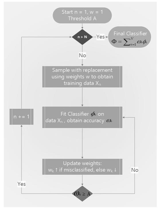
Kearns and Valiant [1989] were among the first to wonder if it was possible to combine poor estimators to get one with great accuracy. Shortly after, Schapire [1990] proved, using what is now known as boosting, that the answer to that question was yes. It generally works like this: First, create one training set using random sampling with replacement and some sample weights (initialized with uniform weights). Second, using the training set, fit one estimator. Third, if the single estimator achieves an accuracy greater than the acceptance threshold (e.g., $50$ in a binary classifier, such that it outperforms chance), it is retained; otherwise, it is rejected. Fourth, give misclassified observations greater weight and properly classified observations less weight. Fifth, continue the preceding procedures until you have $N$ estimators. Sixth, the ensemble prediction is the weighted average of the individual forecasts from the $N$ models, where the weights are the weights of the individual forecasts.

Figure 6.3 shows the AdaBoost decision loop.

are decided by the individual estimators' accuracy There are several boosting algorithms, one of which is AdaBoost (Geron [2017]). The decision flow of a typical AdaBoost implementation is depicted in Figure $6.3$.

How do bagging versus boosting compete in financial applications?

According to the preceding explanation, there are a few differences between boosting and bagging:

• Individual classifiers are fitted in sequential order.

• Underperforming classifiers are eliminated.

Visit https://quantdare.com/what-is-the-difference-between-bagging-and-boosting/ for a graphic explanation of the distinction. - Each iteration weights observations differently.

• The ensemble forecast is a weighted average of the individual learners' predictions.

The significant advantage of boosting is that it minimizes both volatility and bias in forecasts. Correcting bias, on the other hand, comes at the expense of an increased risk of overfitting. Bagging is typically superior to boosting in financial applications. Overfitting addresses are bagged, while underfitting ones are boosted. Because of the low signal-to-noise ratio, it is easy to overfit an ML system to financial data, making overfitting a more significant risk than underfitting. Furthermore, bagging may be parallelized, whereas boosting follows a sequential execution.

What is the role of parallelism in the scalability of the model?

As you may know, several prominent ML methods need to scale better with sample size. SVMs (support vector machines) are a prime example. If you fit an SVM on a million observations, it may take time for the algorithm to converge. Even after convergence, there is no guarantee that the solution is a global optimum or not overfit.

One practical solution is to create a bagging algorithm in which the basis estimator is from a class that does not scale well with sample size, such as SVM. We shall enforce a strict early termination condition while defining that base estimator. For example, with sklearn's SVM implementation, you may set the max iter option to a low number, such as 1E5 iterations. The default parameter is max iter=-1, which instructs the estimator to conduct iterations until errors fall below a threshold. You might also increase the tolerance level using the tol argument, which has a default value of tol=1E-3. Either of these two settings will cause a premature shutdown. With analogous parameters, such as the number of levels in an RF (max depth) or the least weighted percentage of the sum total of weights (of all the input samples) necessary to be at a leaf node, you can halt other algorithms early.

Because bagging techniques may be parallelized, we are breaking down a substantial sequential work into several smaller ones that can be done concurrently. Of course, early halting increases the variance of the individual base estimator outputs; however, this increase can be more than compensated by the variance reduction associated with the bagging procedure. By adding additional independent base estimators, you can regulate the decrease. Bagging enables you to obtain rapid and robust estimates on exceedingly large datasets when used in this manner.