Feature Importance

why repeating of backtest may fail?

One of the most common errors in financial research is taking some data, running it through an ML algorithm, backtesting the predictions, and repeating the process until a nice-looking backtest appears. Such pseudo-discoveries abound in academic journals, and even significant hedge funds are prone to falling into this trap. It makes no difference if the backtest is an out-of-sample walk-forward. The fact that we are repeating a test on the same data will almost certainly result in a false discovery. This methodological error is so well-known among statisticians that the American Statistical Association warns against it in its ethical guidelines (American Statistical Association [2016], Discussion #4). It usually takes around 20 iterations to find a (false) investment strategy with a standard significance level (false positive rate) of 5%.

It's easy to overfit a backtest!

A fascinating aspect of the financial industry is that many experienced portfolio managers (including those with a quantitative background) need to be aware of how simple it is to overfit a backtest. The purpose of this article is to explain one of the analyses that must be performed before performing any backtest.

Assume you are given a pair of matrices $(X, y)$ containing features and labels for a specific financial instrument. We can fit a classifier on $(X, y)$ and evaluate the generalization error through a purged $\mathrm{k}$-fold cross-validation (CV). Assume we have a good performance. The next question is to determine what factors led to that performance. We could incorporate attributes that improve the signal responsible for the classifier's predictive capability. We could remove some features that simply add noise to the system. Notably, comprehending the significance of a feature uncovers the proverbial black box. We can gain insight into the classifier's identified patterns if we understand the information source required. This is one of the reasons why ML skeptics overemphasize the black box mantra. Yes, the algorithm learned without our intervention (that is the whole point of ML!) in a black box, but that doesn't mean we can't (or shouldn't) look at what the algorithm has discovered. Hunters do not eat everything their intelligent dogs retrieve for them, do they?

Once we've determined which characteristics are essential, we can learn more by conducting experiments. Are these characteristics important all the time, or only in certain situations? What causes a shift in importance over time? Are those regime shifts predictable? Are those crucial characteristics applicable to other related financial instruments? Do they apply to different asset classes? What are the most essential attributes of all financial instruments? What features have the highest rank correlation across the entire investment universe? This is a far superior method of researching strategies than the ineffective backtest cycle. Let me state one of the most important lessons I hope you take away from this book:

"Backtesting is not a research tool. Feature importance is."

-Marcos López de Prado

What is the substitution effect and how it affects on feature importance results?

A replacement effect occurs in this context when the projected relevance of one trait is diminished by the existence of other related features. Substitution effects are the ML equivalent of what statistics and econometrics term "multi-collinearity." One method for dealing with linear substitution effects is to do PCA on the raw features before performing feature significance analysis on the orthogonal features. For more information, see Belsley et al. [1980], Goldberger [1991, pp. 245-253], and Hill et al. [2001].

How Substitution Effect may affect feature importance methods

It is helpful to distinguish between feature-importance methods based on whether or not substitution effects are present.

Mean Decrease Impurity

Mean decrease impurity (MDI) is a quick, explanatory-importance (IS) method unique to tree-based classifiers such as RF. At each decision tree node, the selected feature splits the subset it received so that impurity is decreased. Therefore, we can derive how much of the overall impurity decrease can be assigned to each feature. And given that we have a forest of trees, we can average those values across all estimators and rank the features accordingly. See Louppe et al. [2013] for a detailed description. There are some important considerations you must keep in mind when working with MDI:

1. Masking effects occur when tree-based classifiers systematically ignore some features in favor of others. To avoid them, set max features =int (1) when using sklearn's RF class. In this way, only one random feature is considered per level.

   • Every feature is given a chance (at some random levels of some random trees) to reduce impurity.

   • Make sure that features with zero importance are not averaged since the only reason for a 0 is that the feature was not randomly chosen. Replace those values with np. nan.

2. The procedure is obviously IS. Every feature will have some importance, even if it has no predictive power.

3. MDI cannot be generalized to other non-tree-based classifiers.

4. By construction, MDI has the excellent property that features importances add up to 1, and every feature importance is bounded between 0 and 1.

5. The method does not address substitution effects in the presence of correlated features. MDI dilutes the importance of substitute features because of their interchangeability: The importance of two identical features will be halved as they are randomly chosen with equal probability.

6. Strobl et al. [2007] show that MDI is biased towards some predictor variables. White and Liu [1994] argue that, in the case of single decision trees, this bias is due to an unfair advantage given by popular impurity functions toward predictors with many categories.

is Loading ...

MDI feature importance computed on a synthetic dataset

Sklearn's RandomForest class implements MDI as the default feature importance score. This choice is likely motivated by the ability to compute MDI on the fly, with minimum computational cost.

Implementation of MDI Feature Importance

In the RiskLabAI's Julia library, the MDI feature importance is implemented using the featureImportanceMDI function. This function takes 2 inputs:

• classifier (the classifier to fit and prediction),
• featureNames (the feature names),

Similarly, in RiskLabAI's python library, the function feature_importance_MDI does the job.

View More: Julia | Python

Mean Decrease Accuracy

Mean decrease accuracy (MDA) is a slow, out-of-sample method. First, it fits a classifier; second, it derives its performance OOS according to some performance score (accuracy, negative log-loss, etc.); third, it permutates each column of the features matrix $(X)$, one column at a time, deriving the performance OOS after each column's permutation. The importance of a feature is a function of the loss in performance caused by its column's permutation. Some relevant considerations include the following:

1. This method can be applied to any classifier, not only tree-based classifiers.

2. MDA is not limited to accuracy as the sole performance score. For example, in the context of meta-labeling applications, we may prefer to score a classifier with F1 rather than accuracy. That is one reason a better descriptive name would have been "permutation importance." When the scoring function does not correspond to a metric space, MDA results should be used as a ranking.

3. Like MDI, the procedure is also susceptible to substitution effects in the presence of correlated features. Given two identical features, MDA considers one redundant to the other. Unfortunately, MDA will make both features appear outright irrelevant, even if they are critical.

4. Unlike MDI, it is possible that MDA concludes that all features are unimportant. That is because MDA is based on OOS performance.

5. The CV must be purged and embargoed.

is Loading ...

MDA feature importance computed on a synthetic dataset

we will implement MDA feature importance with sample weights, with purged $\mathrm{k}$-fold $\mathrm{CV}$, and with scoring by negative log-loss or accuracy. It measures MDA importance as a function of the improvement (from permutating to not permutating the feature), relative to the maximum possible score (negative log-loss of 0 , or accuracy of 1). In some cases, the improvement may be negative, meaning that the feature is detrimental to the ML algorithm's forecasting power.

Implementation of MDA Feature Importance

In the RiskLabAI's Julia library, the MDA feature importance is implemented using the featureImportanceMDA function. This function takes 6 inputs:

• classifier (the classifier to fit and prediction),
• X (the features matrix),
• y (the labels vector),
• nSplits (the cross-validation number of splits),
• scoreSampleWeights (the sample weights for scoring step),
• trainSampleWeights (the sample weights for training step).

Similarly, in RiskLabAI's python library, the function feature_importance_MDA does the job.

View More: Julia | Python

Methods Without Substitution Effects

Substitution effects can lead us to discard essential features that are redundant. This is not generally a problem in prediction, but it could lead us to wrong conclusions when trying to understand, improve, or simplify a model. For this reason, the following single feature importance method can complement MDI and MDA well.

Single Feature Importance

Single feature importance (SFI) is a cross-section predictive-importance (out-of-sample) method. It computes the OOS performance score of each feature in isolation. A few considerations:

1. This method can be applied to any classifier, not only tree-based classifiers.

2. SFI is not limited to accuracy as the sole performance score.

3. Unlike MDI and MDA, no substitution effects occur since only one feature is considered at a time.

4. Like MDA, it can conclude that all features are unimportant because performance is evaluated via OOS CV. The main limitation of SFI is that a classifier with two features can perform better than the bagging of two single-feature classifiers. For example, (1) feature B may be helpful only in combination with feature A; or (2) feature B may help explain the splits from feature A, even if feature B alone is inaccurate. In other words, standard effects and hierarchical importance are lost in SFI. One alternative would be to compute the OOS performance score from subsets of features, but that calculation will become intractable as more features are considered. next part demonstrates one possible implementation of the SFI method.

is Loading ...

SFI feature importance computed on a synthetic dataset

Implementation of SFI Feature Importance

In the RiskLabAI's Julia library, the SFI feature importance is implemented using the featureImportanceSFI function. This function takes 7 inputs:

• classifier (the classifier to fit and prediction),
• X (the features matrix),
• y (the labels vector),
• nSplits (the cross-validation number of splits),
• scoreSampleWeights (the sample weights for scoring step),
• trainSampleWeights (the sample weights for training step).
• scoring (classifier scoring measure).

Similarly, in RiskLabAI's python library, the function feature_importance_SFI does the job.

View More: Julia | Python

Orthogonal Features

As argued in Section 8.3, Substitution effects dilute the importance of features measured by MDI while significantly underestimating the importance of features measured by MDA. Before applying MDI and MDA, orthogonalize the features as a partial solution. Although an orthogonalization procedure such as principal components analysis (PCA) does not prevent all substitution effects, it should reduce the impact of linear substitution effects.

Consider a stationary feature matrix $\left\{X_{t, n}\right\}$ with observations $t=1, \ldots, T$ and variables $n=1, \ldots, N$: We compute the standardized features matrix $Z$, such that $Z_{t, n}=\sigma_{n}^{-1}\left(X_{t, n}-\mu_{n}\right)$, where $\mu_{n}$ is the mean of $\left\{X_{t, n}\right\}_{t=1, \ldots, T}$ and $\sigma_{n}$ is the standard deviation of $\left\{X_{t, n}\right\}_{t=1, \ldots . T}$. We compute the eigenvalues $\Lambda$ and eigenvectors $W$ such that $Z^{\prime} Z W=W \Lambda$, where $\Lambda$ is a $N \times N$ diagonal matrix with main entries sorted descendingly, and $W$ is a $N \times N$ orthonormal matrix. We calculate the orthogonal features as $P=Z W$. The orthogonality of the features can be verified by noting that $P^{\prime} P=W^{\prime} Z^{\prime} Z W=W^{\prime} W \Lambda W^{\prime} W=\Lambda$.

For two reasons, the diagonalization is performed on $Z$ rather than $X$: (1) Centering the data ensures that the first principal component is oriented correctly in the observation's primary direction. It is analogous to including an intercept in linear regression; (2) re-scaling the data causes PCA to concentrate on explaining correlations rather than variances. With re-scaling, the first principal components would be dominated by the columns of $X$ with the most significant variance, and we would learn more about the structure or relationship of the variables.

next part finds the fewest orthogonal features that explain at least $95$ of $Z$ variance.

Implementation of Orthogonal Features Computation

In the RiskLabAI's Julia library, the orthogonal features is implemented using the orthogonalFeatures function. This function takes 2 inputs:

• X (the features matrix),
• varianceThreshold (the threshold for explained variance filtering),

Similarly, in RiskLabAI's python library, the function orthogonal_features does the job.

View More: Julia | Python

Working with orthogonal features provides two additional benefits in addition to addressing substitution effects: (1) Orthogonalization can also be used to reduce the dimensionality of the feature matrix $X$ by removing features with low eigenvalues. This usually accelerates the convergence of ML algorithms; (2) the analysis is performed on features designed to explain the data structure.

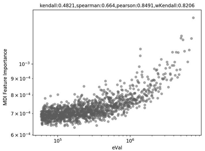
Let me emphasize the latter point. The risk of overfitting is a recurring theme throughout the novel. Even if the pattern is a statistical fluke, ML algorithms will always identify it. Always be wary of ostensibly essential characteristics discovered by any approach, including MDI, MDA, and SFI. Assume you use PCA to generate orthogonal features. Without knowing the labels, your PCA analysis decided that certain features are more "principal" than others (unsupervised learning). That is, PCA has ranked features without any possibility of categorization overfitting. When your MDI, MDA, or SFI analysis identifies the same features as most significant (using label information) as PCA picked as primary (ignoring label information), it confirms evidence that the ML method's pattern is not wholly overfitted. If the features were completely random, the PCA ranking would be unrelated to the feature significance ranking. The scatter plot of eigenvalues associated with an eigenvector ($x$-axis) combined with MDI of the feature related to an eingenvector is shown in Figure $8.1$. (y-axis). The Pearson correlation is $0.8491$ (p-value less than 1E-150), indicating that PCA effectively detected and rated relevant features without overfitting.

The figure Log-log scatter plot of eigenvalues (x-axis) and MDI levels (y-axis).

I find computing the weighted Kendall's tau between the feature importances and their associated eigenvalues handy (or, equivalently, their inverse PCA rank). The closer this number is to one, the more consistent the relationship between PCA rating and feature significance ranking is. One reason to favor weighted Kendall's tau over regular Kendall's tau is that we want to prioritize rank concordance among the most important attributes. We are less concerned with rank concordance among unimportant (presumably noisy) characteristics. For the sample in Figure $8.1$, the hyperbolic-weighted Kendall's tau is $0.8206$.

Parallelized vs. Stacked Feature Importance

There are at least two research methodologies for determining feature significance. To begin, we create a dataset $\left(X_{i}, y_{i}\right)$ for each security $i$ in an investing universe $i=1, \ldots, I$ and extract the feature significance in parallel for each security $i$. For example, indicate the relevance of feature $j$ on instrument $i$ according to criterion $k$ as $\lambda_{i, j, k}$. Then we can integrate all of the findings from the universe to calculate the combined $\Lambda_{j, k}$ relevance of feature $j$ according to criteria $k$. Features essential across a wide range of instruments are more likely to be related to an underlying phenomenon, especially when there is a strong rank correlation across the criteria. Exploring the theoretical process that makes these traits predictive could be worthwhile. The essential advantage of this strategy is that it can be parallelized, which makes it computationally quick. A downside is that significant characteristics may shift ranks among instruments due to substitution effects, raising the variance of the predicted $\lambda_{i, j, k}$. This disadvantage becomes quite negligible if we average $\lambda_{i, j, k}$ across instruments for a sufficiently big investment universe.

Another option is what I call "features stacking." It entails stacking all datasets $\left\{\left(\tilde{X}_{i}, y_{i}\right)\right\}_{i=1, \ldots, I}$ into a single merged dataset $(X, y)$, where $\tilde{X}_{i}$ is a converted instance of $X_i$. (e.g., standardized on a rolling trailing window). The goal of this transformation is to achieve some degree of distributional homogeneity, $\tilde{X}_{i} \sim X$. Under this technique, the classifier must concurrently learn which attributes are more significant across all instruments, as if the entire investing universe were a single instrument. Stacking features has the following advantages: The classifier will be fit on a much larger dataset than in the parallelized (first) approach. The importance is derived directly, and no weighting scheme is required for combining the results. Conclusions are more general and less biased by outliers or overfitting. Because importance scores are not averaged across instruments, substitution effects will not dampen those scores.

I typically favor feature stacking, not just for feature significance but also whenever a classifier can be fitted on a group of instruments, even for model prediction. This decreases the possibility of overfitting an estimator to a specific instrument or short dataset. The biggest downside of stacking is that it consumes a lot of memory and resources; however, here is where a solid understanding of HPC methods comes in help.